Consuming REST JSON APIs From Excel
[Excel, WebAPI, REST]
So today I wanted to see if Excel could natively consume JSON APIs.
So I fired up Excel 2019 and went to the obvious place to find it:

From Online Sources looks like a good candidate.

Nope.
How about From Other Sources?

Nothing seems to stand out here.
It is definitely not OData.
Maybe From Web?
The tool-tip seems to suggest otherwise - web page implies to pull HTML content.

Surely Microsoft Excel 2019, which I believe is the latest, can consume a JSON API!
Turns out it can.
THE TOOLTIP FOR FROM WEB IS MISLEADING!
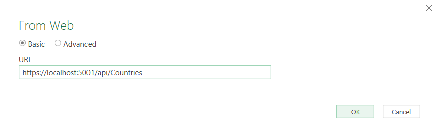
Click it anyway and you will get this prompt:

Paste your URL endpoint there and click OK.
Excel will try to connect and parse the data

It then launches a tool named Power Query.
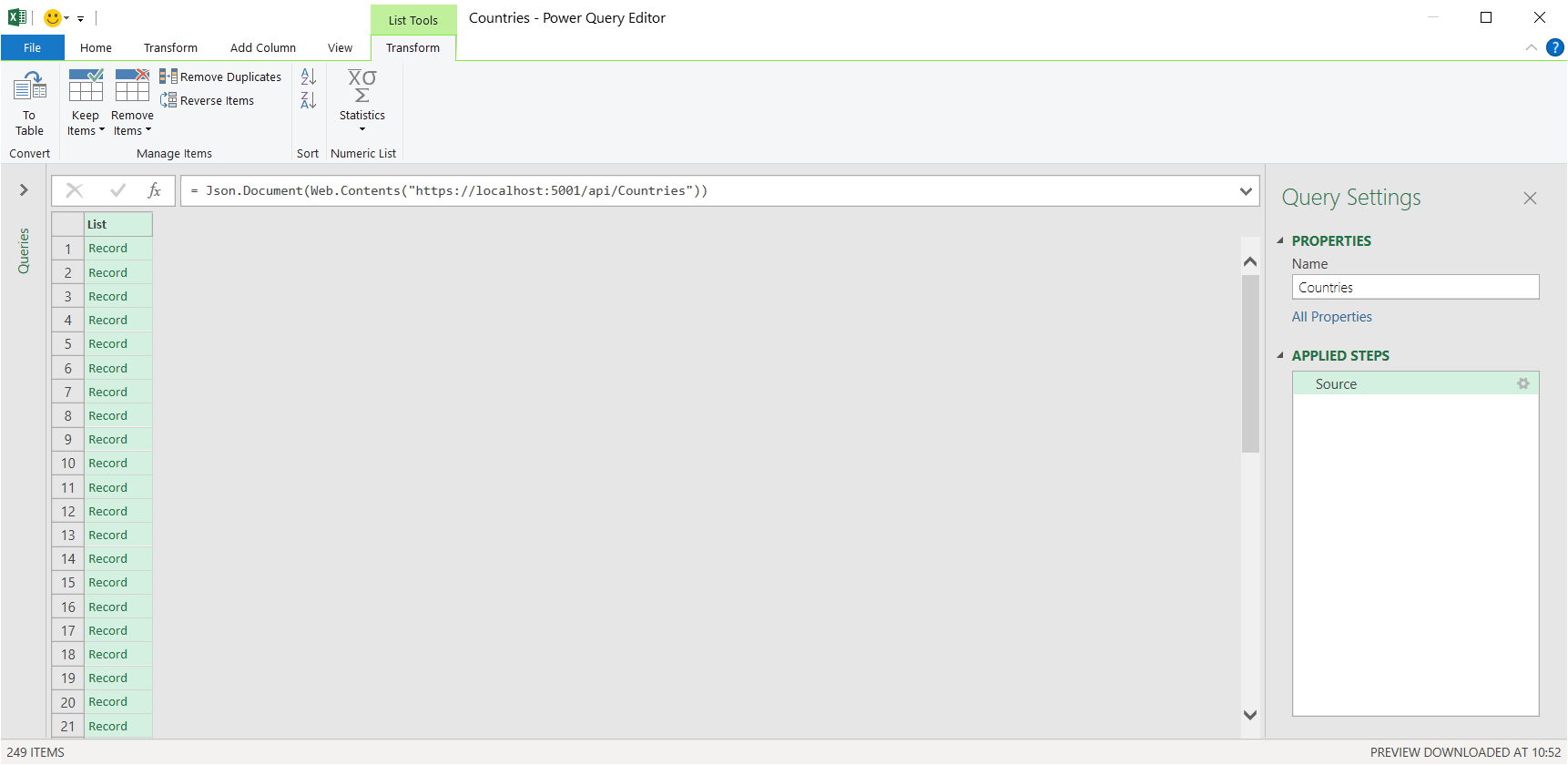
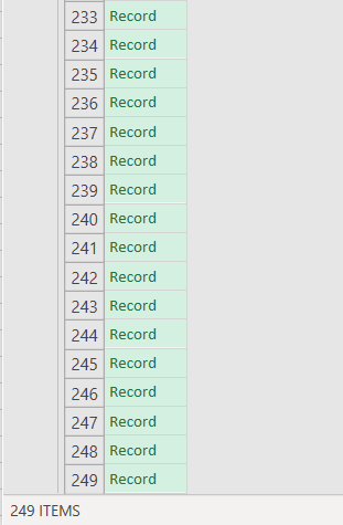
Now I happen to know that this endpoint gives a list of country objects, and that there are 249 of them.
If I scroll down I can confirm this.
If I click on any of the records, Excel expands it.

So it is pulling down the data!
The next step is to instruct Excel how to display it. While it is technically correct that each entry is an object, we want to represent the data as rows.
On the task-pane on your right, click on Source to go back to our original view.
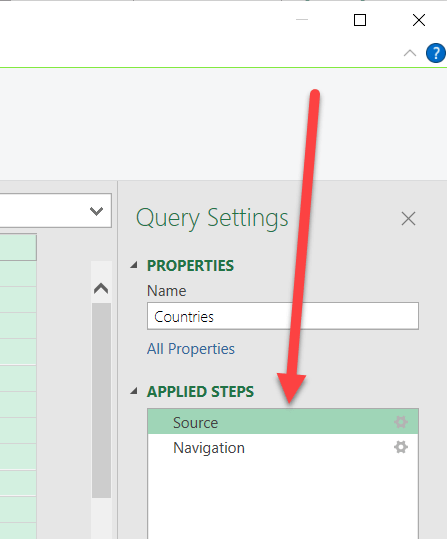
You should go back to this:

To convert this to tabular format, click the button To Table on the menu bar.

You may get this prompt:
Remember when we expanded one of the records? Excel thinks we might want that as part of our workflow.
We don’t.
For now let us go ahead and Insert.
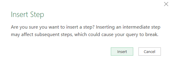
Next we get this prompt.

Click OK.
You will then be returned to this view.

It may look like nothing has changed but something has. Look closely at the column header.
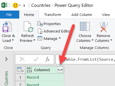
Click on that and you will get a list of the fields in the response.

I don’t want countryID, but I want the others.
Say Insert again to the prompt and we get the following:

We are almost there but there are a couple of things:
First, the column1 prefix is noise. We can get rid of it.
On the task-pane on your right, click the tiny gear icon for the Expanded Column 1 step.

On the resulting screen, remove the caption. You can also change your mind about the fields that you want to see.
The data should now look like this:

While we are at it, we can click the icon on the left and delete the step we took to view a single record

The next problem is the currency column. This appears to be another record.
We can also expand those to view the individual items as columns..
Click this icon on the header:

You should get a choice of columns to view.

I want to see the currency name, ISO Code and Numeric Code only, so I deselect the rest.
This time I want the column name as a prefix so I don’t mix up the currency name and the country name.
This is the resulting data now.

Note the column headers now reflect what we want to see.
What we are viewing here is actually a preview, and in fact you can refresh it at any time by clicking Refresh Preview (if the source data changes while you are configuring the data source.)

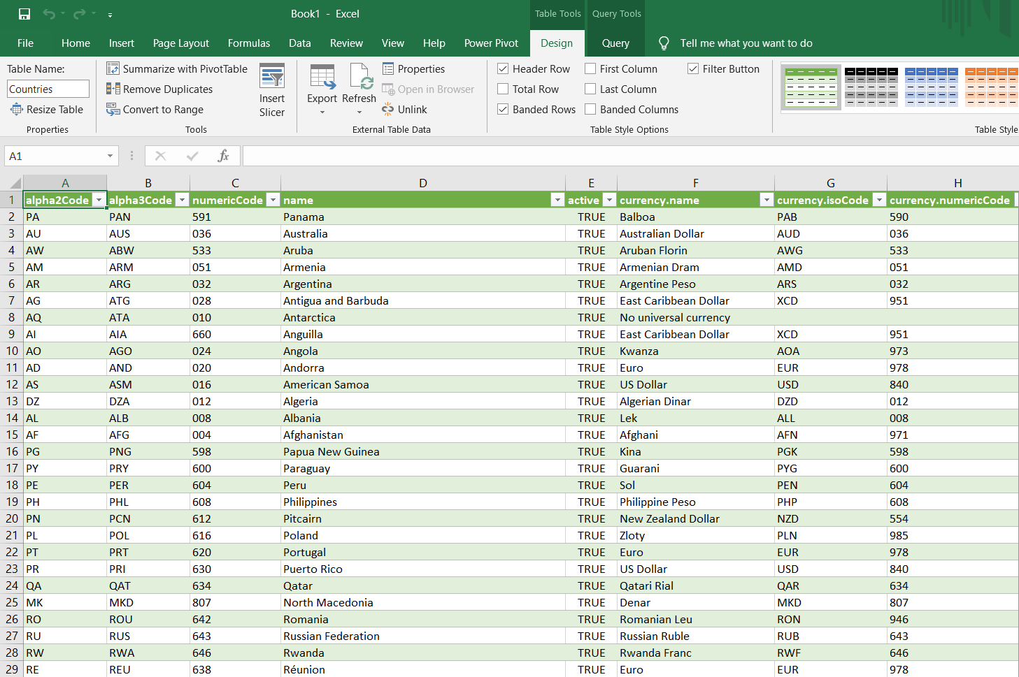
The final step is to get this data back into Excel. Click Close & Load

Our data is now loaded into Excel, beautifully formatted as a table.
You can refresh this data from Excel at anytime by going to the Data pane and clicking Refresh All

Happy hacking!